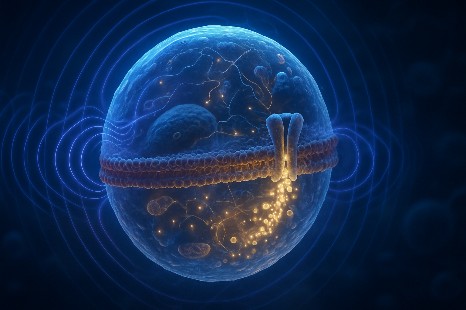
Frequency-Dependent Biological Responses: Unveiling the Potential of Electromagnetic Stimulation in Living Systems

Introduction: Revisiting the Concept of Frequency and Resonance in Electromagnetic Exposure

Biological systems exhibit a diverse range of electromagnetic sensitivities. Cellular activities such as ion transport, membrane-voltage maintenance, protein conformational changes, radical chemistry, gene regulation, and intercellular signaling can all be influenced by electromagnetic fields under appropriate conditions. The central question, however, is not simply whether electromagnetic fields affect biology. It is whether living systems distinguish among frequencies in a reproducible way and whether cells possess a characteristic biological “resonance frequency.”

A universal cellular resonance frequency has not been established. This conclusion is important because the word resonance is often used broadly in discussions of bioelectromagnetics. In physics, resonance generally describes an enhanced response when a periodically driven system is matched to a natural frequency or characteristic relaxation time. A mechanical oscillator, for example, can display a sharply defined resonance when the driving frequency approaches its natural frequency. Biological systems are different. A cell is a warm, aqueous, chemically active, structurally heterogeneous system with many coupled time scales rather than one isolated oscillator. Its responses may depend on membrane charging, ion-channel gating, calcium buffering, enzyme kinetics, receptor desensitization, cytoskeletal motion, transcriptional delays, and circadian or metabolic state.

Consequently, a frequency-dependent response does not automatically demonstrate resonance. A response may instead reflect:

the filtering properties of a membrane or tissue;
the time constant of an ion channel or receptor;
a threshold for electrical excitation;
a frequency-dependent change in induced electric field;
nonlinear rectification of an alternating signal;
beat frequencies or amplitude modulation;
heating or thermal gradients;
synchronization or desynchronization of an intracellular oscillator;
or a narrow experimental “window” created by several interacting variables.

The outcome also depends on field amplitude, polarization, waveform, duty cycle, pulse duration, modulation depth, static magnetic-field background, tissue geometry, electrode configuration, temperature, oxygenation, cell density, and exposure history. A nominal frequency such as 50 Hz or 1 MHz is therefore incomplete as a biological exposure description. Two experiments using the same carrier frequency can produce different biological effects if one uses a continuous sine wave and the other uses short pulses with a 50% duty cycle and strong amplitude modulation.

A useful framework is to treat electromagnetic exposure as a multidimensional input:

[ \mathcal{E}={f,; E_{\mathrm{rms}},; B_{\mathrm{rms}},; \text{waveform},; \text{modulation},; \text{duration},; \text{geometry},; \text{background conditions}}. ]

Here, (f) is frequency, (E_{\mathrm{rms}}) is electric-field strength, and (B_{\mathrm{rms}}) is magnetic-field strength. Biological interpretation requires connecting these external quantities to the field actually present at the membrane, organelle, or tissue target. This is a central objective for rigorous biophysical research, including the Quantum Melanin Research Foundation’s interest in mechanisms that can be stated explicitly and tested through reproducible measurements.

Decoding Biophysical Mechanisms: Electromagnetic Field Effects on Cellular Systems

Electrical Excitability and Membrane Voltage

Mammalian cells maintain membrane potentials through unequal ion distributions and selective membrane permeability. A typical resting potential is approximately (-60) to (-90) mV in neurons and skeletal muscle cells, while many non-excitable cells exhibit values closer to (-20) to (-50) mV. These voltages arise primarily from potassium, sodium, chloride, and calcium gradients maintained by ion pumps and channels. The sodium–potassium ATPase, for example, exports three sodium ions and imports two potassium ions per ATP molecule, contributing both to concentration gradients and to the net electrical polarization of the membrane.

The lipid bilayer is electrically insulating relative to the surrounding aqueous cytoplasm and extracellular fluid. A simplified membrane model treats it as a capacitor in parallel with ion-conducting resistive pathways. The membrane charging time is approximately

[ \tau_m=R_m C_m, ]

where (R_m) is membrane resistance and (C_m) is membrane capacitance. A common specific membrane capacitance is roughly (1,\mu\text{F}/\text{cm}^2). For a small cell, the whole-cell capacitance may be on the order of 10–100 pF, although the effective resistance can vary by orders of magnitude depending on cell type and channel activity. This gives membrane time constants ranging from less than a millisecond to tens or hundreds of milliseconds.

That time constant creates frequency-dependent electrical filtering. If an applied field changes slowly compared with (\tau_m), the membrane can charge and discharge substantially during each cycle. At much higher frequencies, the membrane voltage may not follow the external field as effectively. This does not mean that high-frequency fields are biologically inert; rather, the dominant coupling mechanism may shift from direct membrane polarization to dielectric heating, induced currents, molecular dipole interactions, or other processes.

Strong, spatially varying electric fields can directly stimulate excitable tissue. The most relevant quantity for nerve and muscle excitation is often the electric field component along the axon or excitable membrane, particularly its spatial gradient. A uniform electric field may polarize different parts of a cell in opposite directions, whereas a field gradient can create a depolarizing region sufficient to initiate an action potential.

Time-varying magnetic fields can produce electric fields according to Faraday’s law:

[ \nabla \times \mathbf{E}=-\frac{\partial \mathbf{B}}{\partial t}. ]

For an idealized sinusoidal magnetic field perpendicular to a circular region of radius (r),

[ B(t)=B_0\sin(\omega t), ]

the induced azimuthal electric-field amplitude is approximately

[ E_{\mathrm{ind}}(r)=\frac{r}{2}\omega B_0 ]

inside the region, where (\omega=2\pi f). This equation is simplified, but it illustrates why frequency, magnetic amplitude, and geometry must be reported together.

Worked example. Suppose a sinusoidal magnetic field has an amplitude of (B_0=100,\mu\text{T}=1.0\times10^{-4},\text{T}), a frequency of (50) Hz, and acts over a circular region with (r=0.10) m. Then:

[ E_{\mathrm{ind}}\approx \frac{0.10}{2}(2\pi \times 50)(1.0\times10^{-4}) \approx 1.6\times10^{-3},\text{V/m}. ]

The estimated induced field is therefore about (1.6) mV/m. This is far below the electric fields commonly used for direct peripheral-nerve stimulation, which are often in the range of several volts per meter or greater at the relevant neural structures, depending on pulse shape, electrode geometry, and target orientation. The calculation does not prove that weaker fields have no biological effects; it establishes the scale that any proposed mechanism must accommodate.

A second example demonstrates the effect of frequency. Keeping (B_0=100,\mu\text{T}) and (r=0.10) m constant while increasing frequency from 50 Hz to 1 kHz increases the idealized induced field by a factor of 20, from approximately (1.6) mV/m to (31) mV/m. However, the biological response still depends on whether the induced field is aligned with a sensitive cellular structure, whether it exceeds an excitation threshold, and whether the waveform is continuous or pulsed.

At low frequencies, magnetic fields can penetrate tissue relatively effectively because tissue is not strongly shielded from slowly varying magnetic flux. Electric fields behave differently: conductive tissue redistributes charge and can attenuate or distort externally applied fields. In culture systems, the plastic dish, medium depth, electrode placement, and return-current path may therefore determine the actual field experienced by cells. This is one reason that field mapping and numerical modeling are important rather than optional additions.

Calcium: A Sensitive Mediator of Electromagnetic Signals

Calcium ions are particularly important in discussions of electromagnetic biology because calcium concentration changes can amplify small upstream signals. Cytosolic free calcium is commonly maintained near approximately (50)–(150) nM in resting cells, whereas extracellular calcium is typically around (1)–(2) mM. The resulting concentration ratio can exceed (10^4), creating a strong electrochemical driving force. Calcium is also stored in the endoplasmic reticulum and mitochondria, which act as intracellular reservoirs and sinks.

A transient increase from 100 nM to 1 µM represents a tenfold change in free cytosolic calcium, even though the absolute number of calcium ions involved may be small relative to the total ionic content of the cell. Such transients can activate calmodulin, protein kinase pathways, phosphatases, contractile proteins, vesicle fusion, mitochondrial metabolism, and transcription factors. Calcium can therefore function as a biochemical gain stage: a modest change in membrane voltage or receptor activity may trigger a much larger downstream response.

This amplification does not establish that calcium ions directly resonate with a particular electromagnetic frequency. Instead, frequency dependence may emerge from the kinetics of the systems controlling calcium. For example, a voltage-gated calcium channel may open in response to depolarization, inactivate over milliseconds, and recover over a longer interval. A train of pulses delivered faster than the recovery time may produce less current per pulse, whereas pulses spaced at an intermediate interval may maximize calcium entry. The apparent optimum frequency would then be a property of channel kinetics and cellular feedback, not a universal calcium resonance.

Calcium responses can also involve intracellular release. A small influx through the plasma membrane may trigger calcium-induced calcium release from the endoplasmic reticulum in some cell types. Conversely, mitochondrial uptake and endoplasmic-reticulum buffering can suppress or reshape the signal. The measured endpoint may therefore depend on whether an experiment records:

total cellular calcium;
cytosolic free calcium;
calcium near the plasma membrane;
mitochondrial calcium;
endoplasmic-reticulum depletion;
the frequency of calcium spikes;
or the integrated calcium exposure over time.

These endpoints are not interchangeable. A field could leave the average calcium concentration unchanged while altering pulse timing, spatial localization, or oscillation frequency.

Distinctions Among Frequency, Waveform, and Exposure History

Frequency is only one descriptor of a time-varying field. A complete exposure report should include peak amplitude, root-mean-square amplitude, phase relationships, waveform shape, rise and fall time, pulse width, repetition rate, duty cycle, modulation frequency, modulation depth, exposure duration, and the field orientation relative to the biological target.

For a sinusoidal field,

[ B(t)=B_0\sin(2\pi ft), ]

the root-mean-square value is

[ B_{\mathrm{rms}}=\frac{B_0}{\sqrt{2}}. ]

Thus, a field with a 1 mT peak amplitude has an RMS amplitude of approximately 0.707 mT. Comparing this with a reported value of 1 mT RMS without conversion would create a 41% amplitude error.

Waveform can be equally consequential. A square wave with the same nominal frequency and peak amplitude as a sine wave contains odd harmonics at (3f), (5f), (7f), and higher frequencies. A 10 Hz square-wave pulse train may therefore expose cells to substantial spectral components at 30, 50, and 70 Hz, depending on rise time and duty cycle. Short pulses additionally contain broad high-frequency spectral components. Claims about a “10 Hz effect” are consequently incomplete unless the pulse shape and spectrum are specified.

Modulation creates another layer. A carrier at (f_c) with amplitude modulation at (f_m) contains sidebands near (f_c-f_m) and (f_c+f_m). If a biological system responds to the envelope rather than the carrier, the relevant frequency may be the modulation frequency. If it responds to tissue heating, the carrier and average power may matter more. If nonlinear ion-channel processes rectify the signal, the mean or low-frequency component can become important even when the applied field is centered around zero.

Exposure history also matters. Cells can adapt, desensitize, or enter a different physiological state after an initial stimulus. A 30-minute continuous exposure is not equivalent to thirty 1-minute exposures separated by 1-minute recovery periods. A useful dose description may include both cumulative duration and the temporal arrangement of pulses. For a pulsed field, the duty cycle is:

[ D=\frac{t_{\mathrm{on}}}{t_{\mathrm{on}}+t_{\mathrm{off}}}. ]

A pulse sequence with (t_{\mathrm{on}}=1) ms and (t_{\mathrm{off}}=9) ms has a 10% duty cycle. Its average power, heating potential, and biological effect can differ substantially from a continuous field with the same peak amplitude.

Temperature must be measured rather than assumed. A change of only (0.5)–(1^\circ\text{C}) can affect membrane fluidity, enzyme rates, ion-channel kinetics, and oxygen consumption. In radiofrequency studies, specific absorption rate (SAR) is often used to quantify energy deposition:

[ \mathrm{SAR}=\frac{\sigma |E|^2}{\rho}, ]

where (\sigma) is tissue conductivity, (E) is the electric-field magnitude, and (\rho) is mass density. At lower frequencies, induced-current density and electric-field distributions may be more informative than SAR alone. No single dosimetric quantity is adequate across all frequency ranges.

Addressing the Energy-Scale Dilemma

The energy of a photon is

[ E=hf, ]

where (h=6.626\times10^{-34},\text{J}\cdot\text{s}). At 50 Hz:

[ E\approx 3.3\times10^{-32},\text{J}, ]

which corresponds to approximately (2.1\times10^{-13}) eV per photon. By comparison, thermal energy at room temperature is

[ k_BT\approx 4.1\times10^{-21},\text{J}\approx 0.026,\text{eV}. ]

The thermal energy scale is therefore roughly eleven orders of magnitude larger than the energy of an individual 50 Hz photon. At 1 MHz, the photon energy is still only about (4\times10^{-9}) eV, far below (k_BT).

This comparison rules out simplistic explanations based on the absorption of isolated low-frequency photons producing chemical bond changes. It does not, by itself, rule out all weak-field effects. Classical electromagnetic fields can influence charged particles collectively, and biological systems can amplify small perturbations through threshold processes and feedback. Examples include membrane excitability, enzyme cascades, radical-pair chemistry, and synchronization of pre-existing oscillations.

However, any proposed weak-field mechanism must identify a plausible coupling pathway and show that it exceeds noise, thermal fluctuations, and competing physiological processes. A credible mechanism should specify the field at the molecular target, the interaction energy or force, the relevant relaxation time, and the amplification route from the primary physical perturbation to the measured endpoint. “Resonance” should not be used as a substitute for this chain of reasoning.

Historical Insights: Calcium Efflux and Biological "Windows"

The Pioneering Bawin–Adey Studies

The studies associated with Bawin, Adey, and collaborators reported frequency-dependent changes in calcium efflux from neural tissues exposed to weak amplitude-modulated radiofrequency fields. These experiments became influential because they appeared inconsistent with a simple monotonic model in which biological response increases continuously with field intensity. Instead, responses were reported within particular combinations of carrier frequency, modulation frequency, field strength, and exposure conditions.

The concept of a biological “window” describes a response that is stronger within a restricted parameter range and weaker outside it. In a two-dimensional frequency–amplitude plot, such a response might resemble a band or island rather than a straight threshold boundary. For example, a hypothetical experiment might show an increased calcium-efflux signal at modulation frequencies between 10 and 20 Hz, no effect at 1 Hz or 100 Hz, and a diminished response when amplitude is increased tenfold. Such behavior could reflect nonlinear channel kinetics, adaptation, interference among pathways, or a genuine narrow operating range.

The early findings were significant because they encouraged researchers to investigate modulation and waveform instead of focusing only on carrier frequency and average intensity. They also highlighted a recurring difficulty: when effects are small, a response can be sensitive to temperature, medium composition, electrode currents, magnetic background, vibration, lighting, and the physiological condition of the tissue.

Statistical Validation and Methodological Rigor

Subsequent work, including studies associated with Blackman and colleagues, emphasized the statistical and experimental complexity of characterizing frequency-dependent calcium responses. A “window” requires more than finding one statistically significant frequency. It requires demonstrating that:

the response is reproducibly localized to a defined region of parameter space;
neighboring frequencies were tested rather than omitted;
the effect survives correction for multiple comparisons;
sham-exposed samples were handled identically;
field amplitude and temperature were independently verified;
the result is not caused by apparatus artifacts;
the response has a plausible biological time course; and
independent laboratories can reproduce the effect.

The multiple-comparison problem is particularly important. If 100 frequencies are tested at a nominal significance level of (p<0.05), approximately five false-positive results may be expected by chance even when no frequency has a true effect. A statistically credible frequency-window study therefore requires a prespecified analysis plan, correction for multiple testing, adequate replication, and preferably an independent validation set.

A practical design might use a logarithmic or otherwise justified frequency grid, for example 1, 3, 10, 30, 100, and 300 Hz, followed by finer spacing around any apparent response. Each frequency should be tested in randomized order, with blinding where feasible. The study should report the number of biological replicates, technical replicates, confidence intervals, effect size, and raw distributions rather than relying only on a bar graph of group means.

Lessons from Early Studies

The calcium-efflux literature offers several lasting lessons. First, biological responses can be nonlinear and can depend on combinations of parameters rather than on frequency alone. Second, subtle effects are unusually vulnerable to hidden variables. Third, replication is not merely a final confirmation; it is part of the mechanism-validation process.

A modern replication should use calibrated field probes, three-dimensional field modeling where appropriate, sham coils or matched apparatus controls, continuous temperature monitoring, magnetic shielding or characterization of background fields, and independent measurement of electrode polarization or leakage currents. Cell viability, pH, osmolality, dissolved gases, and medium temperature should be recorded because each can influence calcium handling.

It is also useful to distinguish between exploratory and confirmatory frequency scans. Exploratory screens are appropriate for locating candidate windows but produce hypotheses that must be tested in a separate experiment. Confirmatory studies should freeze the exposure parameters before data collection and use an independent biological batch. This separation reduces the risk that a frequency is selected because it happened to show the largest response in the initial dataset.

Theoretical Mechanisms: Bridging Electromagnetic Influence with Cellular Responses

Interactions with Voltage-Gated Calcium Channels

Voltage-gated calcium channels are plausible transducers because their open probability depends strongly on membrane voltage. A field-induced membrane perturbation of only a few millivolts could, in principle, alter channel gating if it occurs at the channel’s sensitive membrane domain and at a sufficiently rapid or appropriately timed interval. In practice, the required field depends on channel subtype, membrane orientation, resting potential, channel density, and the noise generated by spontaneous channel opening and closing.

A simplified gating model describes the probability of channel opening as a voltage-dependent function:

[ P_{\mathrm{open}}(V)=\frac{1}{1+\exp[-(V-V_{1/2})/k]}, ]

where (V_{1/2}) is the voltage at which half the channels are activated and (k) describes voltage sensitivity. If (k=6) mV, a 6 mV depolarization can produce a substantial change in activation probability near (V_{1/2}). But a field applied across a cell does not necessarily generate 6 mV across the channel’s gating region. The induced potential may be distributed across the whole cell, membrane, extracellular medium, and neighboring structures.

For a spherical cell in a uniform low-frequency electric field, the transmembrane potential can be approximated in simplified form as scaling with field magnitude and cell radius:

[ \Delta V_m \sim \alpha E a\cos\theta, ]

where (a) is cell radius, (\theta) is the angle relative to the field, and (\alpha) depends on membrane and medium properties. For a cell with (a=10,\mu\text{m}) in a field of (1,\text{V/m}), the characteristic induced voltage scale is on the order of micovolts to tens of microvolts, depending on frequency and assumptions. That is much smaller than the tens of millivolts typically associated with action-potential initiation, although local geometries, cell processes, tissue interfaces, and strong field gradients can increase polarization.

This scale comparison is essential. A proposed channel-mediated mechanism must explain whether the effect arises from direct gating, altered local electric fields near channel proteins, modulation of channel phosphorylation, or an indirect pathway. It should also predict how the response changes with channel blockers, extracellular calcium concentration, membrane potential, temperature, and genetic removal of the channel subtype.

Intracellular Mechanism Dynamics

Electromagnetic exposure could potentially influence intracellular calcium dynamics through several routes. A primary effect at the plasma membrane might alter calcium influx. A secondary effect could change phospholipase C signaling, inositol trisphosphate production, or receptor sensitivity, leading to endoplasmic-reticulum calcium release. Mitochondria may then buffer the signal, alter ATP production, or generate reactive oxygen species. The final measured response could thus be several steps removed from the initial electromagnetic interaction.

A useful experimental strategy is to measure multiple stages of the pathway in parallel. For example:

membrane potential can be measured with voltage-sensitive dyes or electrophysiology;
calcium influx can be separated from internal release using calcium-free extracellular medium or channel inhibitors;
endoplasmic-reticulum release can be assessed with compartment-specific indicators;
mitochondrial calcium and membrane potential can be measured separately;
downstream kinase activation can be quantified by phosphorylation assays;
transcriptional effects can be evaluated only after controlling for earlier calcium and stress responses.

Time resolution helps distinguish mechanisms. A change beginning within milliseconds of field onset is more compatible with direct electrical or channel-mediated coupling than a transcriptional response that emerges after 30–120 minutes. Conversely, a delayed response may reflect secondary signaling, altered metabolism, or gene regulation rather than direct electromagnetic detection.

Exploring Radical Chemistry and Reactive Oxygen Species

Radical-pair mechanisms provide a theoretically interesting route for weak magnetic-field sensitivity. In a radical pair, two unpaired electrons can exist in singlet or triplet spin states. Magnetic interactions can alter singlet–triplet interconversion, which may change the chemical products formed when the radicals recombine. This mechanism is particularly relevant to chemical systems involving flavins, cryptochromes, and other redox-active molecules.

The challenge is to establish physiological relevance. A radical-pair hypothesis must identify the molecular radical pair, its lifetime, its spin interactions, the relevant magnetic-field range, and the predicted change in reaction yield. Radical lifetimes may range from nanoseconds to microseconds or longer, while magnetic-field effects depend on hyperfine couplings, exchange interactions, and molecular orientation. The presence of a magnetic response in a purified chemical system does not automatically demonstrate that the same effect occurs in a living cell at a biologically meaningful magnitude.

Reactive oxygen species are similarly ambiguous endpoints. A small change in radical chemistry may be amplified through redox-sensitive signaling, but ROS can also increase because of heating, mitochondrial stress, altered oxygenation, mechanical disturbance, or assay artifacts. Fluorescent ROS indicators can themselves be affected by light exposure, dye concentration, oxidation state, and cellular loading. Therefore, ROS claims should use multiple probes, positive and negative controls, and independent measures such as antioxidant sensitivity, mitochondrial function, and direct chemical assays.

Melanin-rich systems may be of interest in this context because melanin contains stable organic radicals and can participate in redox reactions, charge transport, and energy dissipation. Yet the presence of paramagnetic centers alone does not establish a frequency-selective biological detector. A rigorous hypothesis would need to specify whether the relevant interaction involves spin state, proton transfer, charge separation, radical lifetime, or another molecular property, and then connect that property to a measurable cellular outcome.

Testing Hypothetical Scenarios

Low-field frequency hypotheses can be tested through staged experimental designs. A first-stage screen might expose several cell types to a prespecified range of frequencies and amplitudes while measuring calcium, membrane voltage, temperature, viability, and ROS simultaneously. A second-stage experiment would focus on candidate windows and test whether the effect changes predictably with channel blockers, calcium-free medium, antioxidants, or genetic perturbation.

Consider a hypothetical study examining a 1–300 Hz magnetic field. Suppose the field amplitude is (100,\mu\text{T}) RMS, exposure lasts 20 minutes, temperature remains within (0.05^\circ\text{C}) of sham controls, and cells are tested at 1, 3, 10, 30, 100, and 300 Hz. If calcium fluorescence increases only at 30 Hz, the next experiment should not merely repeat 30 Hz. It should test nearby frequencies such as 20, 25, 30, 35, 40, and 50 Hz, along with amplitude levels such as 10, 30, 100, and 300 (\mu\text{T}). This determines whether the effect is a narrow frequency window, an amplitude threshold, or a broad response centered on a particular time scale.

A genuine mechanism should also yield perturbation predictions. If voltage-gated calcium channels are required, a channel blocker should reduce the effect. If internal stores are responsible, extracellular calcium removal may not eliminate the initial response. If the response is caused by heating, a sham condition with matched temperature should reproduce it. If amplitude modulation is essential, replacing the modulated waveform with an unmodulated carrier at the same RMS power should abolish or reduce the response.

The strongest evidence would combine dose–response data, temporal dynamics, pharmacological intervention, genetic manipulation, physical modeling, and independent replication. Statistical significance alone is insufficient if the effect is small, variable, or disconnected from a plausible transduction pathway.

Evaluating Current Evidence: Drawing from Established Facts to Future Directions

Well-Established Findings

Several principles of electromagnetic interaction with biological systems are firmly established. Strong static magnetic fields exert forces and torques on magnetic materials and can affect certain experimental procedures. Time-varying magnetic fields induce electric fields. Strong electric fields can stimulate nerves and muscles. Radiofrequency fields can deposit energy and produce heating. Ionizing electromagnetic radiation, at sufficiently high photon energies, can produce electronic excitation and molecular damage. These effects have well-characterized physical mechanisms and can often be predicted from field strength, geometry, tissue properties, and exposure duration.

Medical technologies demonstrate that electromagnetic stimulation can be biologically effective when parameters are appropriately chosen. Transcranial magnetic stimulation uses rapidly changing magnetic fields to induce electric fields in the brain. Peripheral nerve stimulation uses controlled electric currents. Deep brain stimulation applies electrical pulses directly through implanted electrodes. Radiofrequency ablation deliberately generates heat. Photobiomodulation uses red or near-infrared light under defined conditions, with mechanisms involving absorption, redox signaling, mitochondrial activity, and tissue optics.

These examples support the general proposition that biological systems respond to electromagnetic inputs. They do not establish that every frequency has a specific receptor or that weak environmental fields produce equivalent effects. The evidence is strongest when field intensity, target location, and coupling mechanism are clearly defined.

Areas of Ambiguity

Ambiguous findings are common when exposure fields are weak, biological endpoints are variable, and the number of tested frequencies is large. Differences among laboratories may arise from cell-line drift, passage number, confluence, medium composition, temperature control, coil placement, shielding, background magnetic fields, instrument noise, or differences in endpoint analysis.

Epidemiological associations require similar caution. Associations between extremely low-frequency magnetic-field exposure and childhood leukemia have been reported in some analyses, particularly at higher residential exposure categories, but observational evidence does not by itself establish causality. Potential confounding, exposure misclassification, selection effects, and the absence of a firmly established mechanism remain important considerations. A credible causal interpretation would require consistency across populations, a dose-related pattern, temporal plausibility, biological coherence, and experimental support.

Another ambiguity concerns “nonthermal” exposure. The absence of measurable bulk heating does not mean the absence of all energy transfer, but it also does not prove a biologically active nonthermal mechanism. Localized interactions, transient currents, and chemical amplification are possible in principle, yet they must be quantitatively demonstrated rather than inferred from the word nonthermal.

Prerequisites for Reliable Frequency-Dependent Findings

A robust claim of frequency dependence should satisfy several methodological requirements:

Complete exposure characterization: report frequency, peak and RMS field strength, waveform, modulation, duty cycle, pulse width, polarization, orientation, duration, and static background fields.
Field mapping: measure the field at the cell or tissue location, not only at the generator or coil.
Thermal monitoring: record temperature continuously or at sufficiently short intervals to detect transient heating.
Dosimetric modeling: estimate induced electric field, current density, SAR, or another physically relevant quantity.
Appropriate controls: include sham exposure, apparatus controls, temperature-matched controls, and, where relevant, electrode-current controls.
Randomization and blinding: randomize exposure order and blind sample identity during endpoint analysis when practical.
Broad frequency testing: test neighboring frequencies and amplitudes rather than reporting only the strongest condition.
Adequate replication: distinguish technical repeats from independent biological replicates.
Multiple endpoints: pair a primary response such as calcium fluorescence with viability, membrane voltage, ROS, or pathway-specific markers.
Mechanistic perturbation: use blockers, knockouts, antioxidants, calcium removal, or altered membrane potential to test causal predictions.
Independent validation: reproduce the finding in a separate experiment, biological batch, and preferably laboratory.
Transparent statistics: prespecify primary outcomes, correct for multiple comparisons, report effect sizes and confidence intervals, and provide raw or individual-level data.

A worked example illustrates why frequency should be treated as an integrative parameter. Suppose two experiments both report a 10 Hz magnetic exposure at (1) mT. In Experiment A, the field is a continuous sine wave with 1 mT RMS amplitude. In Experiment B, it is a 1 mT peak square pulse train with a 10% duty cycle, amplitude-modulated at 10 Hz, and accompanied by a 0.4°C temperature rise. These are not equivalent exposures. Their RMS amplitudes, harmonic content, average power, induced electric fields, and thermal histories differ. Treating them as the same “10 Hz, 1 mT” condition would make biological comparison unreliable.

What If? Exploring Promising Applications and Directions

If reproducible frequency windows are eventually identified, electromagnetic interventions could become more selective. Neurological applications might use pulse timing matched to neuronal excitability or network oscillations. Cellular engineering could potentially exploit field parameters that influence calcium dynamics, differentiation, wound repair, or metabolic activity. Drug delivery and tissue regeneration may benefit from combining electromagnetic stimulation with materials that concentrate fields or convert them into local mechanical, thermal, optical, or chemical signals.

Such applications require more than identifying an effective frequency. The molecular transducer must be understood. A practical therapy would need a defined target, a predictable dose, a measurable biological response, and a safety margin separating the desired effect from unwanted excitation, heating, oxidative stress, or tissue damage.

Future studies may combine electrophysiology, live-cell imaging, optogenetic or chemogenetic controls, nanoscale field measurements, computational electrodynamics, and single-cell transcriptomics. These tools can help determine whether apparently variable responses arise from a small responsive subpopulation, synchronized cellular states, or an average effect across all cells. In melanin-containing systems, measurements of radical concentration, redox state, charge mobility, optical absorption, and spin behavior could test whether melanin functions as a relevant electromagnetic transducer under defined conditions rather than merely serving as a descriptive association.

The most productive direction is therefore neither to dismiss all weak-field effects nor to assume that every reported frequency window represents a biological resonance. It is to define the coupling pathway, quantify the field at the target, test competing explanations, and reproduce the result under independently controlled conditions.

Key Takeaways

Biological responses to electromagnetic fields are well established in several exposure regimes, but they vary with frequency, amplitude, waveform, geometry, and exposure history.
A universal cellular resonance frequency has not been identified; many apparent frequency windows may reflect membrane filtering, channel kinetics, nonlinear signaling, modulation, or experimental artifacts.
Calcium is a powerful and sensitive biological mediator, but a calcium response does not by itself prove direct electromagnetic resonance.
Time-varying magnetic fields induce electric fields according to Faraday’s law, and the induced magnitude depends on frequency, field amplitude, spatial scale, and geometry.
ELF photon energies are vastly below thermal energies, so weak-field mechanisms require collective, classical, nonlinear, or chemically amplified coupling rather than single-photon bond breaking.
Historical calcium-efflux studies stimulated valuable research into non-monotonic biological responses but also demonstrated the importance of replication, field characterization, and statistical control.
Voltage-gated calcium channels, intracellular calcium stores, mitochondria, radical-pair chemistry, and melanin-associated redox processes are plausible areas for investigation, not established universal mechanisms.
Reliable frequency-dependent findings require calibrated dosimetry, temperature controls, randomized exposure, broad parameter testing, mechanistic perturbation, transparent statistics, and independent laboratory validation.
Frequency should be treated as one component of a multidimensional exposure profile rather than as an isolated biological determinant.
Well-defined electromagnetic windows could eventually support targeted applications in neurology, tissue engineering, and cellular modulation, provided that molecular transducers and safety limits are demonstrated.